scqubits, part one: a qubit in five lines
How do you get the spectrum, the wavefunctions, the matrix elements and a coherence estimate for a real circuit, and what is each one for?
About this section: The Workbench: the two programs
Installation first, with the exact error messages you are likely to meet, and a map of where each program’s own documentation lives. Then QuTiP in two topics (objects, then solvers) and scqubits in two (a qubit, then coupled systems and sweeps). The last of them joins the two programs, which is how they are used together. The code is meant to be copied and changed.
See it
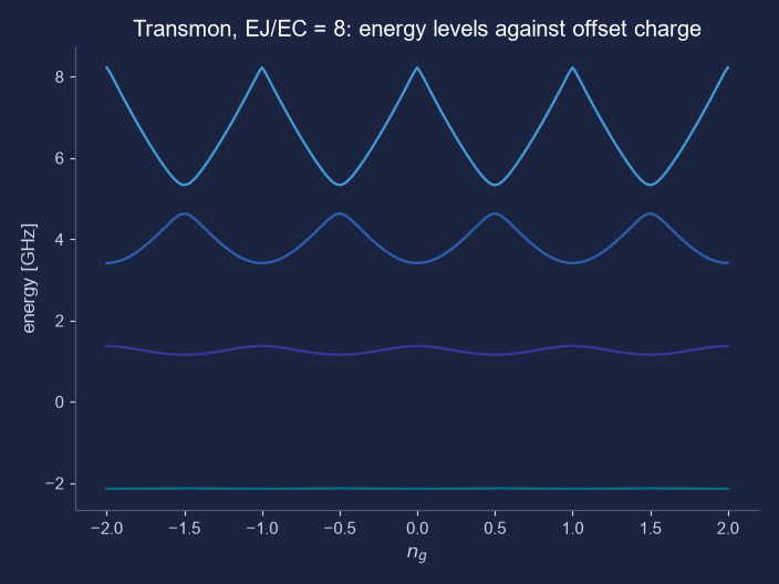
plot_evals_vs_paramvals draws. A transmon with a small EJ/EC of 8, so that the charge dispersion of topic 29 is easy to see: the higher the level, the more it moves when the offset charge changes. The picture is the unretouched output of scqubits 4.3.1 (only its colours were changed to suit this page), made by two lines of the code below.Try it: sweep a parameter and get the line of Python
Choose a qubit and a parameter to sweep and the picture draws itself, as plot_evals_vs_paramvals would. Below it is the single line that makes the same plot in scqubits, with your numbers in it. Switch to the wavefunction view to see the shape of each level in the well, which is what plot_wavefunction shows.
Honest limits: the explorer redraws the diagonalisation of topics 29 and 30 in your browser, not scqubits itself, and agrees with scqubits to twelve digits on the cases in the verifier. For anything but a quick look, run the real package.
The intuition
An scqubits qubit is a small Python object with the circuit’s parameters as attributes: Transmon(EJ, EC, ng, ncut), TunableTransmon(EJmax, EC, d, flux, ng, ncut), Fluxonium(EJ, EC, EL, flux, cutoff), and the flux, cos(2φ) and 0–π qubits. Energies are in GHz (as E/h, the convention of this part), and the last parameter, ncut or cutoff, is how many basis states to keep: the same cutoff of topic 26, and the first thing to vary when you doubt an answer. Change an attribute and the object recomputes, which is what makes a sweep one line.
Five things to ask a qubit. Its levels (eigenvals, E01(), anharmonicity()). Its eigenvectors (eigensys). Its operators in its own eigenbasis, and the table of their matrix elements (matrixelement_table). Its wavefunctions in the phase variable (plot_wavefunction). And how long it lives, from a loss model (t1_capacitive and its relatives). The matrix elements are the part newcomers skip and should not: they decide which transitions a drive, a resonator or a neighbouring qubit can cause, and a zero in the table is a selection rule.
Reading the matrix-element table. In the transmon at zero offset charge, the Hamiltonian has a mirror symmetry: levels are either even or odd, alternately. The charge operator is odd, so it connects an even level only to an odd one. The table below has exact zeros at (0, 2) and (1, 3) for that reason, and a small non-zero 0.0395 at (0, 3), which is allowed and is the sign that a transmon is not a perfect oscillator. The strong entries, 1.09, 1.49 and 1.76, grow along the ladder like √n, as they would for the oscillator, but not exactly.
A coherence number is an estimate from a model. t1_capacitive assumes the dielectric around the junction loses energy with a quality factor that you can set; by default it takes the frequency-dependent form of Smith et al. (2020), at 15 mK. The number it returns, 29.1 µs here, is only as good as that assumption, and what scqubits gives you is a way to see how it moves as you change the design, not a measurement of a chip. The check below does the same arithmetic by hand and gets the same answer, which tells you the code does what its documentation says.
The mathematics, as calls
| Call | What it returns |
|---|---|
qubit.eigenvals(evals_count=n) | the n lowest energies, in GHz |
qubit.eigensys(evals_count=n) | those energies and their eigenvectors (columns) |
qubit.E01(), qubit.anharmonicity() | f01 and f12 − f01 |
qubit.matrixelement_table("n_operator", evals_count=n) | ⟨i|n|j⟩ for the n lowest levels, as an array |
qubit.plot_evals_vs_paramvals("ng", values) | a picture of the levels as one parameter changes |
qubit.plot_wavefunction(which=[0, 1, 2]) | |ψ(φ)|² of those levels, drawn at their energies in the potential |
qubit.t1_capacitive(i=1, j=0, T=0.015) | T1 from dielectric loss, in ns for energies in GHz |
qubit.supported_noise_channels() | which loss and dephasing models this qubit has |
The loss model, written out. The transition rate from level 1 to level 0 is Fermi’s golden rule with the charge operator as the noise, Γ = |⟨0|n|1⟩|² S(ω01), and for dielectric loss the spectral density is S(ω) = 2π · 16 EC / Qcap(ω) times thermal factors that equal 1 when ħω ≫ kBT (here ħω/kBT = 18 at 15 mK). With Qcap(ω) = 10⁶ (6 GHz/f)0.7, f01 = 5.68258 GHz and |⟨0|n|1⟩| = 1.0878, the rate is 3.4355 × 10⁻⁵ per ns, so T1 = 29.1 µs. The numbers: levels −12.077, −6.3945, −1.0566, 3.8959 and 8.3416 GHz, f01 = 5.68258 GHz, |⟨0|n|1⟩| = 1.0878 and a capacitive-loss T1 of 29.1 µs, the last reproduced by hand.
Try it in Python. The first lines are the five-line version; the rest is the table, a sweep and the by-hand check. Run on scqubits 4.3.1 with QuTiP 5.2.0, 25 October 2026:
import numpy as np
import scqubits as scq

scq.settings.PROGRESSBAR_DISABLED = True
scq.settings.T1_DEFAULT_WARNING = False

tm = scq.Transmon(EJ=15.0, EC=0.3, ng=0.0, ncut=30)           # GHz; the same transmon as topic 29

print(tm)                                                      # the parameters, in a table
print("levels:", np.round(tm.eigenvals(evals_count=5), 4))
print("E01 =", round(tm.E01(), 5), "GHz; anharmonicity =", round(tm.anharmonicity(), 5), "GHz")

# matrix elements of the charge operator between the lowest levels: a table, with its selection rules
mel = tm.matrixelement_table("n_operator", evals_count=4)
print(np.round(np.abs(mel), 4))

# change a parameter and ask again: a flux-tunable transmon at two fluxes
tt = scq.TunableTransmon(EJmax=40.0, EC=0.3, d=0.0, flux=0.0, ng=0.0, ncut=30)
for flux in (0.0, 0.25):
    tt.flux = flux
    print("flux", flux, "-> E01 =", round(tt.E01(), 4), "GHz")

# a coherence estimate from a loss model. With energies in GHz, times come back in ns.
t1 = tm.t1_capacitive(i=1, j=0, T=0.015)
print("capacitive-loss T1 =", round(t1 / 1000, 1), "microseconds")

# the same number by hand: the loss model of Smith et al. (2020), as scqubits writes it
f01, n01 = tm.E01(), abs(mel[0, 1])
Q = 1e6 * (6.0 / f01) ** 0.7                                   # dielectric quality factor, falling slowly with frequency
rate = 2 * np.pi * 16 * tm.EC * n01 ** 2 / Q                   # per ns; at 15 mK the thermal factors are 1
print("by hand:", round(1 / rate / 1000, 1), "microseconds")
Transmon------------| [Transmon_1]
| EJ: 15.0
| EC: 0.3
| ng: 0.0
| ncut: 30
| truncated_dim: 6
|
| dim: 61
levels: [-12.077 -6.3945 -1.0566 3.8959 8.3416]
E01 = 5.68258 GHz; anharmonicity = -0.34477 GHz
[[0. 1.0878 0. 0.0395]
[1.0878 0. 1.4903 0. ]
[0. 1.4903 0. 1.7552]
[0.0395 0. 1.7552 0. ]]
flux 0.0 -> E01 = 9.4879 GHz
flux 0.25 -> E01 = 7.9269 GHz
capacitive-loss T1 = 29.1 microseconds
by hand: 29.1 microsecondsThe two pictures scqubits makes for this transmon are below. Left, the three lowest wavefunctions sit in the cosine well at their own energies, so that the nodes (zero crossings) are visible: level 0 has none, level 1 has one, level 2 has two. Right, the matrix elements as bars and as a map; the checkerboard of zeros is the selection rule.
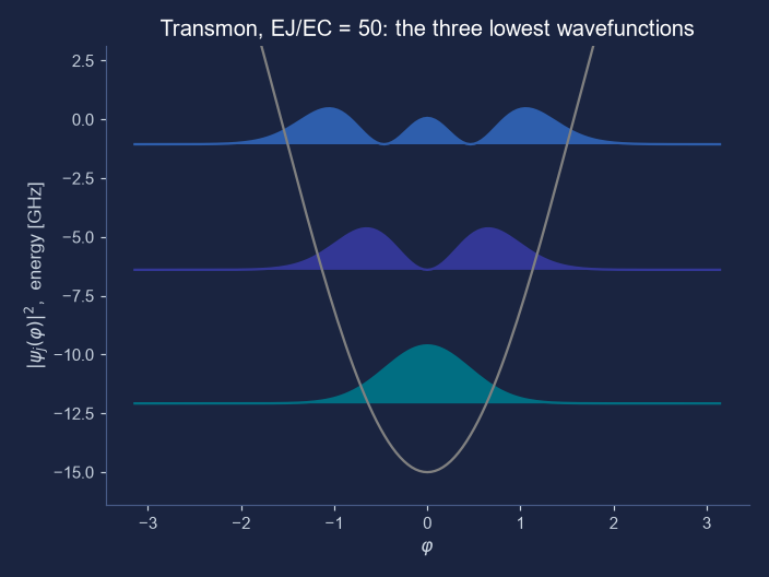
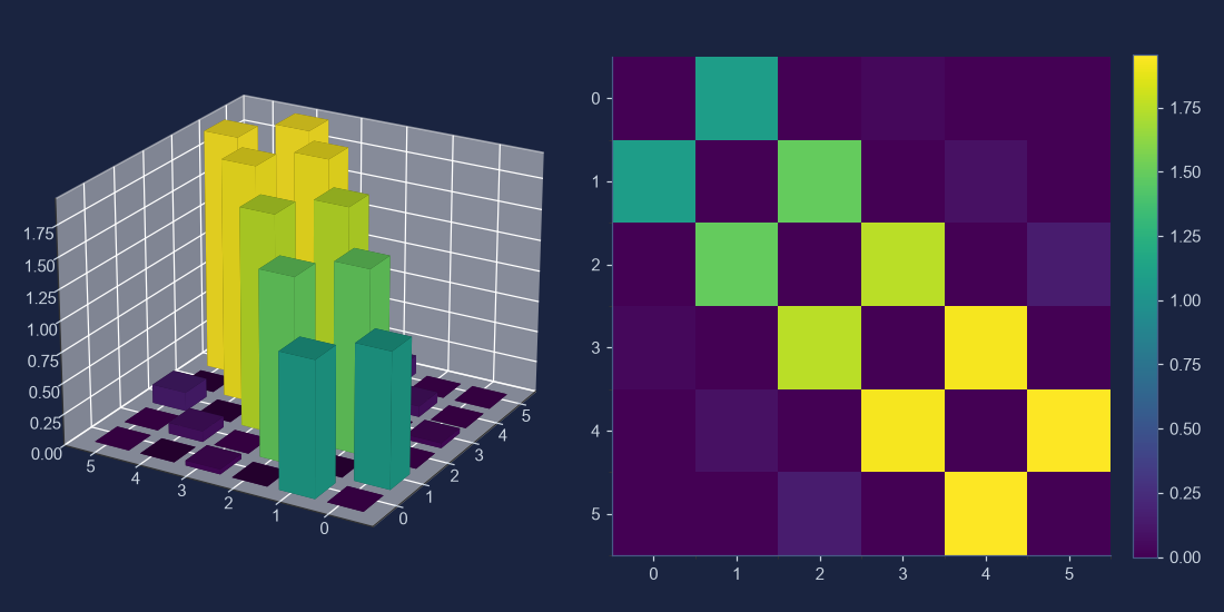
tm.plot_wavefunction(which=[0, 1, 2], mode="abs_sqr") and tm.plot_matrixelements("n_operator", evals_count=6).Where it actually matters
The first thing a design review asks for
Given a layout’s EJ and EC, the first questions are the frequency, the anharmonicity, how sensitive the qubit is to charge (topic 29), and which transitions a given coupling will excite, which is the matrix-element table. A sweep like the one in the picture, repeated over the junction’s variation from the fab, tells you how much the frequency will scatter. scqubits packages that loop; its example notebooks demo_transmon.ipynb, demo_fluxonium.ipynb and demo_noise.ipynb in the scqubits-examples repository are the best next reading. What it does not do is build the circuit from a layout: that is the job of the electromagnetic tools in topic 38, which feed it the two energies.
Check yourself
In a transmon at zero offset charge, the charge-operator matrix element between levels 0 and 2 is exactly zero. Why?
At zero offset charge the Hamiltonian has a mirror symmetry, so each level is even or odd in turn. The table has zeros at (0, 2) and (1, 3) for that reason and a small non-zero 0.0395 at (0, 3), which is allowed.
The tempting wrong answers.
- “The 0 to 2 transition needs two quanta at once, and a charge drive supplies only one at a time.” Picking this counts quanta as if the transmon were an exact oscillator; a parity rule forbids it, and 0 to 3 is small but allowed.
- “The gap between levels 0 and 2 is too large for the drive to bridge, whatever its strength.” Picking this blames the size of the gap; selection rules have nothing to do with energy.
- “It is zero only because of the chosen values E_J = 15 and E_C = 0.3 GHz; other values would give a non-zero element there.” Picking this mistakes a symmetry for an accident: the zero holds for every E_J and E_C at zero offset charge.